2 Simple examples of graphics

2.1 A rectangle inside another one

program example1, file demo.cmd

This program draws a red rectangle in the X11 window, then a blue rectangle inside the first one. It does the same on a Postscript file. Here we don't use any frame. To use this program, when demo.cmd is loaded, type

 - funct -> clear X
 - funct -> example1

:example1
1
1
-1
;
setcolor X red
graphplot X 100 100
graphline X 100 300
graphline X 500 300
graphline X 500 100
graphline X 100 100
;
setcolor X blue
graphplot X 150 150
graphline X 150 250
graphline X 450 250
graphline X 450 150
graphline X 150 150
;

The result is the following figure

2.2 Graphic representation of functions

Program example2, file demo.cmd

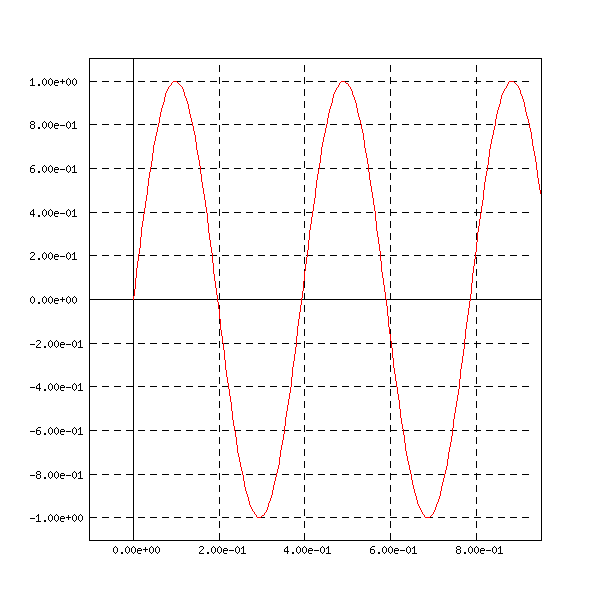
The following program draws the function sin(x) on a window. Of course it is better to use the command funct_plot. To use this program, when demo.cmd is loaded, type

 - funct -> clear X
 - funct -> example2

:example2
1
0
-1
;
;
defframe f
frame f 0 2*pi -1 1 1 .2 
dt=pi/200
;
;
setclip 0.15 0.75 0.1 0.7
setframe X f
setcolor X red
graphplot_c X f 0 0
dt=pi/200
;
do i 0 400
t=i*dt
graphline_c X f t sin(t)
enddo
;
destroy f
; restore the original frame size
setclip 0.15 0.9 0.1 0.9
setcolor X black
;

The result is represented on the following figure

2.3 A complicated picture

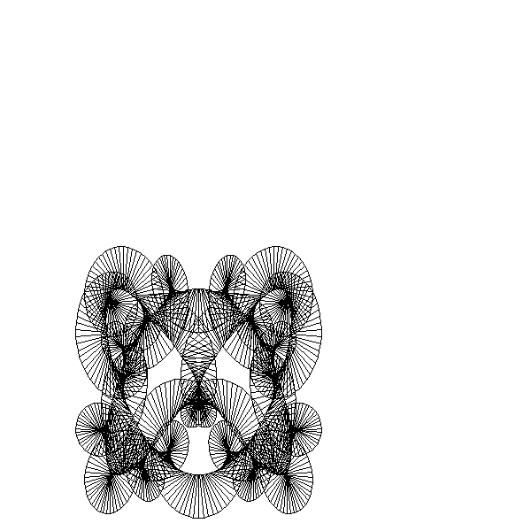
Program lion_X11, file demo.cmd

The following program draws a black picture on a window, with a size determined by the first parameter. Here we don't use any frame. To use this program, when demo.cmd is loaded, type

 - funct -> clear X
 - funct -> lion_X11 .7

:lion_X11
2
0
-1
;
;
@d=pi/500
@t=0
@a=320.
@b=90.
@A=@a
@B=20.
graphplot X @a*#1 @b*#1
;
do i 1 1000
[1
@t=@t+@d
@x=320.+150.*sin(2.*@t)
@y=240.-150.*cos(3.*@t)
@u=@x+50.*sin(20.*@t)
@v=@y-70.*cos(20.*@t)
]
graphline X @a*#1 @b*#1
graphline X @x*#1 @y*#1
graphline X @u*#1 @v*#1
graphline X @A*#1 @B*#1
graphline X @a*#1 @b*#1
graphline X @x*#1 @y*#1
[1
@a=@x
@b=@y
@A=@u
@B=@v
]
enddo
;

The result is represented below

2.4 The same picture inside a frame

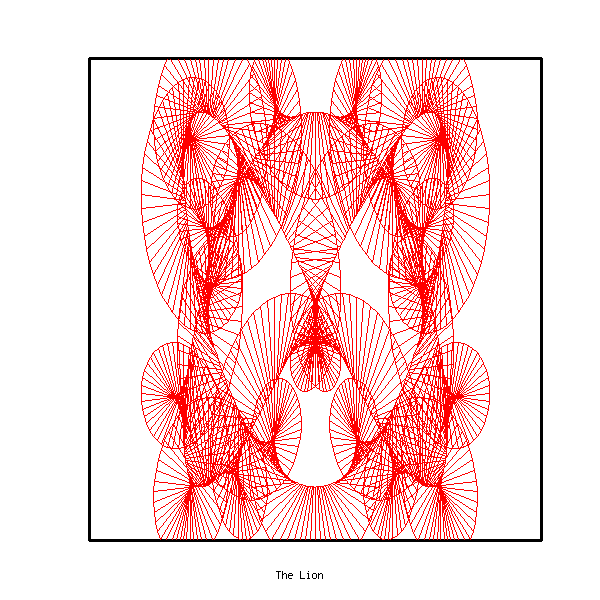
Program lion_X11_c, file demo.cmd

The following program draws the same picture as in the preceeding example, but in red and inside a frame. Only the parts of the picture that are inside the frame will be drawn. The size of the frame is determined by the first parameter. To use this program, when demo.cmd is loaded, type

 - funct -> clear X
 - funct -> lion_X11_c 0.8

:lion_X11_c
2
0
-1
defframe f
frame f 320*(1-#1) 320*(1+#1) 240*(1-#1) 240*(1+#1) 640 480 
setframe X f 
setcolor X red
@d=pi/500
@t=0
@a=320.
@b=90.
@A=@a
@B=20.
graphplot_c X f @a @b
;
do i 1 1000
[1
@t=@t+@d
@x=320.+150.*sin(2.*@t)
@y=240.-150.*cos(3.*@t)
@u=@x+50.*sin(20.*@t)
@v=@y-70.*cos(20.*@t)
]
graphline_c X f @a @b
graphline_c X f @x @y
graphline_c X f @u @v
graphline_c X f @A @B
graphline_c X f @a @b
graphline_c X3 f @x @y
[1
@a=@x
@b=@y
@A=@u
@B=@v
]
enddo
;
destroy f
;

The result is represented here

2.5 Four pictures with different scales

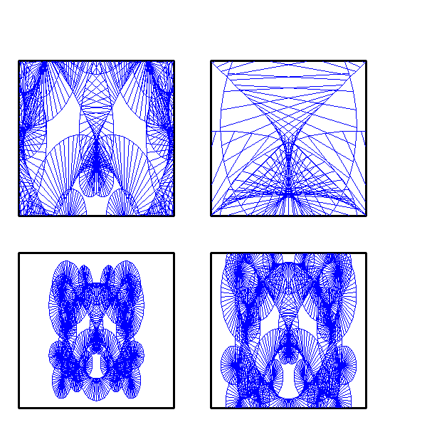
Program lion_X11_c_b, file demo.cmd

The following program draws the same picture in four regions of the image, with different scales. The first parameter determines the size of the 4 frames. This program uses the subprogram lion_plot. To use this program, when demo.cmd is loaded, type

 - funct -> clear X
 - funct -> lion_X11_c_b .9

:lion_X11_c_b
1
0
-1
;
;
defframe f1
defframe f2
defframe f3
defframe f4
frame f1 0 800 0 600 800 600
frame f2 120 680 90 510 800 600
frame f3 240 560 180 420 800 600
frame f4 360 440 240 360 800 600
setclip .05 .45 .05 .45 
setframe X f1 
setclip .55 .95 .05 .45 
setframe X f2 
setclip .05 .45 .55 .95 
setframe X f3 
setclip .55 .95 .55 .95 
setframe X f4 
;
;
setcolor X blue
@d=pi/500
setclip .05 .45 .05 .45 
lion_plot f1
setclip .55 .95 .05 .45 
lion_plot f2
setclip .05 .45 .55 .95 
lion_plot f3
setclip .55 .95 .55 .95 
lion_plot f4
;
destroy f1
destroy f2
destroy f3
destroy f4
;
; restore the original frame size
setclip 0.15 0.9 0.1 0.9
;
;
;
;
:lion_plot
2
0
-1
@t=0
@a=400.
@b=112.
@A=@a
@B=25.
graphplot_c X #1 @a @b
;
do i 1 1000
[1
@t=@t+@d
@x=400.+187.*sin(2.*@t)
@y=300.-187.*cos(3.*@t)
@u=@x+62.*sin(20.*@t)
@v=@y-87.*cos(20.*@t)
]
graphline_c X #1 @a @b
graphline_c X #1 @x @y
graphline_c X #1 @u @v
graphline_c X #1 @A @B
graphline_c X #1 @a @b
graphline_c X #1 @x @y
[1
@a=@x
@b=@y
@A=@u
@B=@v
]
enddo
;

The result is shown below

2.6 Graphic representation of functions - Better way

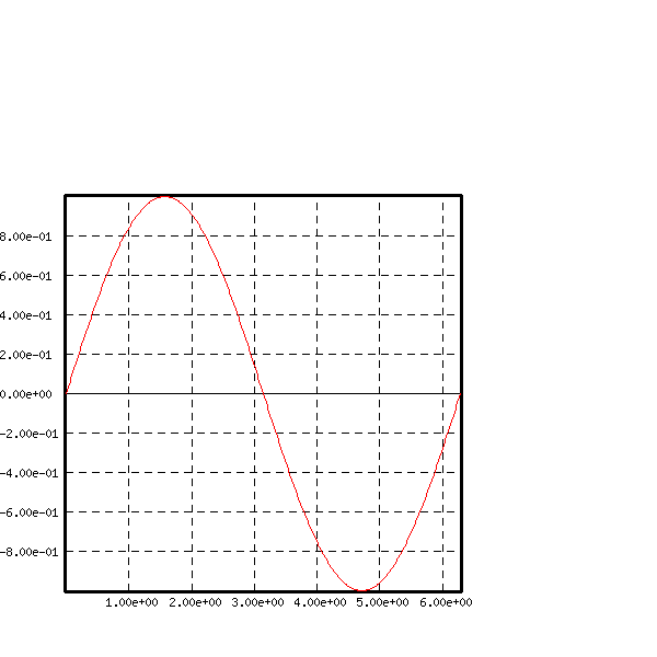
Program Func_draw, file demo.cmd

The following program will plot the function $sin(16x)$ for $x$ between $0$ and $1$ on a window. It uses the command funct_plot. To use this program, when demo.cmd is loaded, type

 - funct -> clear X
 - funct -> Func_draw

:Func_draw
1
0
-1
;
xrange xr 1 1001
fix_xrange xr 0 .001
function F xr
fill_func F sin(16*x)
defframe f
frame f -.1 .95 -1.1 1.1 .2 .2
setframe X f
setcolor X red
funct_plot F X f 0 1 250
destroy f
destroy xr
;

The result is