3 Examples of programs using functions

3.1 Bessel functions and transforms

Program test_bessel, file demo.cmd

It is a test of the Bessel transforms. We use the formula

$$\frac{d}{dx}(x^nj_n(\lambda x)) \ = \ \lambda x^nj_{n-1}(\lambda x).$$

We compute, for $i$ from 0 to 5 the Bessel transform of order $i$ of the function $x^{i+1}$ on the interval $[0,30]$. The result must be the function $3^{i+1}j_{i+1}(3t)/t$. We compute for each $i$ the functions $Gi$ and $GGi$ which are respectively the Bessel transform of order $i$ of the function $x^{i+1}$ and the function $3^{i+1}j_{i+1}(3t)/t$ computed directly.

To run the program, when demo.cmd is loaded, type the commands :

 - funct -> clear X
 - funct -> test_bessel

;------------------------------------------------------------------------
;-------- test program for Bessel transforms ---------------------------- 
;------------------------------------------------------------------------
:test_bessel
1
0
-1
xrange xr 1 1000
fix_xrange xr 0 0.003
xrange xr3 1 1000
fix_xrange xr3 0.001 0.03
;
function n0 xr
fill_func n0 x
def_four tr0 n0 2048
function G0 xr3
def_bes_par zz0 0 400
trans_bessel tr0 zz0 G0
function GG0 xr3
fill_func GG0 3.*jv(1,3.*x)/x
destroy tr0
destroy zz0
;
;
function n5 xr
fill_func n5 x^6
def_four tr5 n5 2048
function G5 xr3
def_bes_par zz5 5 400
trans_bessel tr5 zz5 G5
function GG5 xr3
fill_func GG5 729.*jv(6,3.*x)/x
destroy tr5
destroy zz5
;
;
;
graph_bes 0
color_echo green
echo Hit Enter\n
color_echo black
waitkey 
clear X
echo We do the same ,for i=5, the two functions are plotted on the\n
echo interval [0,30].\n
graph_bes 5
;
destroy xr
destroy xr3
;
;
; subprogram that draws the results
:graph_bes
2
1
-1
fmin=0
fmax=0
min_func G#1
max_func G#1
fmin=fmin_func
fmax=fmax_func
min_func GG#1
max_func GG#1
if> fmin_func-fmin zz
fmin=fmin_func
zz:
if< fmax_func-fmax yy
fmax=fmax_func
yy
defframe f#1
frame f#1 0 30 fmin fmax 5. 9.5*#1-7.5
setframe X f#1
defframe f#1b
frame f#1b 0 5 fmin fmax 2. 9.5*#1-7.5
;
setcolor X blue
funct_plot G#1 X f#1 0 30 1000
setcolor X red
funct_plot GG#1 X f#1 0 30 1000
;
color_echo green
echo Hit Enter\n
color_echo black
waitkey
clear X
setframe X f#1b
setcolor X blue
funct_plot G#1 X f#1b 0 5 1000
setcolor X red
funct_plot GG#1 X f#1b 0 5 1000
destroy f#1
destroy f#1b
echo \n
echo The same result, on [0,5]\n
echo \n
;

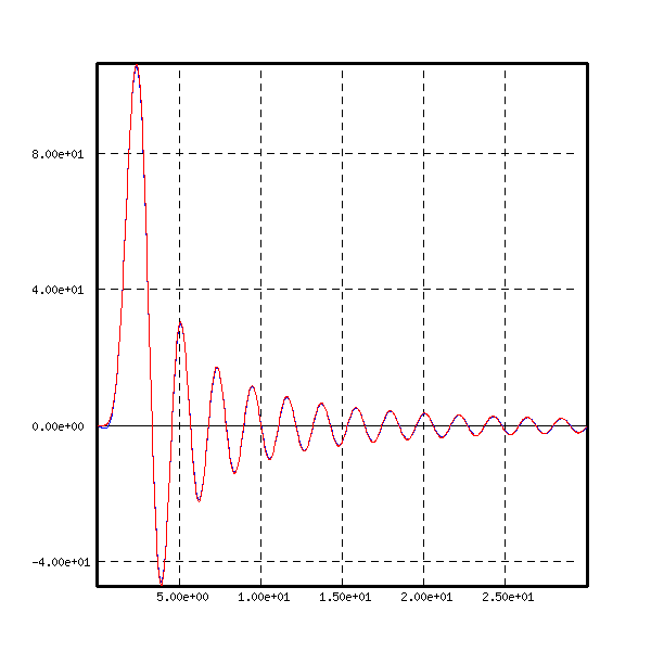
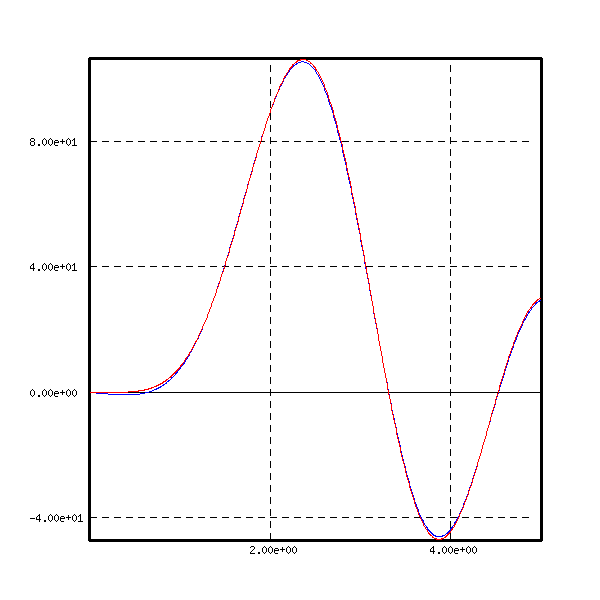
We represent in figure here the case $i=0$. The Bessel transform is in blue, and over it the directly computed formula is in red.

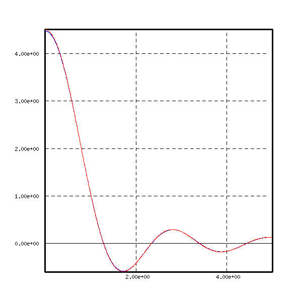
We represent also now the case $i=0$, but we zoom in the interval [0,5].The Bessel transform is in blue, and over it the directly computed formula is in red.

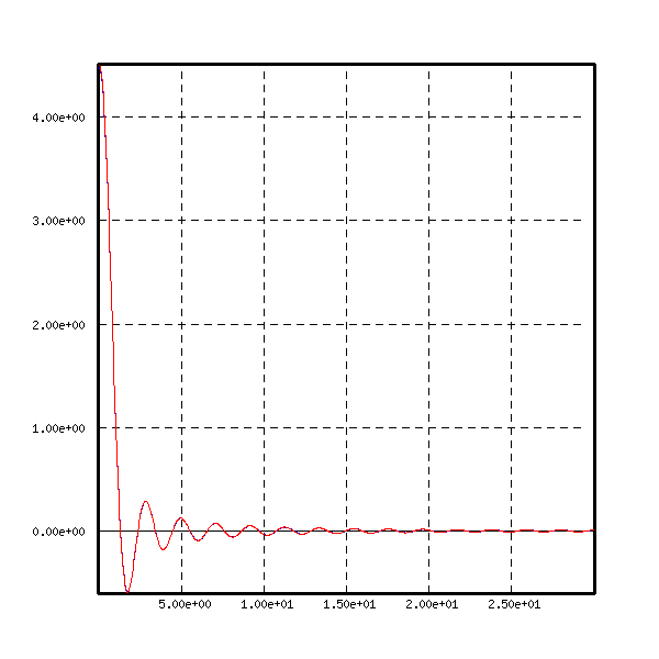
We represent below the case $i=5$. The Bessel transform is in blue, and over it the directly computed formula is in red.

We represent also here the case $i=5$, but we zoom in the interval [0,5]. The Bessel transform is in blue, and over it the directly computed formula is in red.

3.2 Lévy-Khintchin transform

Program Lev_Kh, file demo.cmd

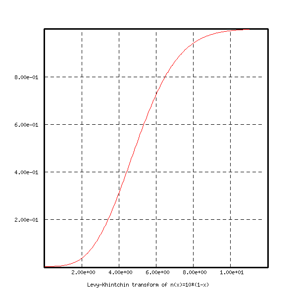
This program computes the Levy-Khintchin transform of then function

$$n(x) \ = \ 10(1-x)$$

for $0\leq x\leq 1$. Recall that this transform is the probability function

$$P(x) \ = \ 1-\frac{2}{\pi} \int_0^\infty \cos(tx)\frac{\sin(tR(t))}{t}e^{-tI(t)}dt$$

where the real functions $R(t)$ and $I(t)$ are respectively the real part and the imaginary part of the Fourier transform of $n$ :

$$R(t)+iI(t) \ = \ \int^\infty_0n(x)e^{itx}dx .$$

To run the program, when demo.cmd is loaded, type the commands :

 - funct -> clear X
 - funct -> Lev_Kh

;------------------------------------------------------------------------
;---------- Levy-Khintchin formula --------------------------------------
; This program computes the Levy-Khintchin transform of the function
; 	n(x) = 10*(1-x),    0 <= x <= 1
; i.e. the probability function with Poisson kernel n(x)
;------------------------------------------------------------------------
:Lev_Kh
1
0
-1
xrange xr 1 1000
fix_xrange xr 0 0.001
function n xr
fill_func n 10*(1-x)
def_four tr1 n 2048
xrange xr1 1 2000
fix_xrange xr1 0 0.0015
function_C fC xr1
trans_four tr1 fC
function fC.r xr1
function fC.i xr1
real fC fC.r
imag fC fC.i
function t xr1
fill_func t x
function R xr1
function I xr1
mul_func fC.r t R
mul_func fC.i t I
function Si xr1
comp_func sin(x) R Si
function Ex xr1
comp_func exp(-x) I Ex
function f2 xr1
div_func Si t f2
val_func fC.r 0
fix_func_R f2 1 func
function f3 xr1
mul_func f2 Ex f3
def_four tr2 f3 2048
xrange xr2 1 4000
fix_xrange xr2 0 0.01
function_C P xr2
trans_four tr2 P
function P.r xr2
function P.i xr2
real P P.r
imag P P.i
val_func P.r 0
function cnst xr2
const_func cnst func
function q xr2
sub_func cnst P.r q
x=2/pi
rmul q x q
val_func q 18
defframe f
frame f 0 12 0 1 2 .2
setframe X f
setcolor X red
funct_plot q X f 0 12 1000
xflush
;
destroy xr
destroy xr2
destroy xr1
destroy tr1
destroy tr2
destroy f
;

The following figure shows the result of the Levy-Khintchin transform.

3.3 Power series

Program test_serieb, file demo.cmd

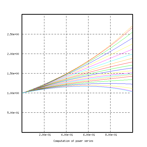
This the program computes the power series

$$\sum_{p=0}^n\frac{c(p)}{p!}x^p ,$$

where $c(p)$ is given by a function or by a formula. We consider the cases

$$c(p) \ = \ \cos(ap^2)$$

and compute the power series for $a=0, 0.5, 1.0, 1.5, ...$ up to $10$. We take $n=20$ and $0\leq x\leq 1$. We have then a good approximation for the complete power series (with $n=\infty$).

To run the program, when demo.cmd is loaded, type the commands :

 - funct -> clear X
 - funct -> test_serieb

;-------------------------------------------------------------------------
;-------- program of computation of a power series -----------------------
; serie F Np c n j
;
; F : real DP function 
; F will contain the sum of (c(p)/p!).x^p  from p=0 to p=n
;
; Np : number of points where the series is computed
; c : if  j==0  it is the function c(p)
;     if  j==1  it is a formula giving c(p) in terms of p
;     if  j==3  this parameter is not used, the program calc_func
;		is called and returns c(p) in the variable 'func'
; n : number of terms
; j : the parameter used previously
;------------------------------------------------------------------------
:serie
6
0
-1
desc_func #1
xrange xr_temp 1 #2
fix_xrange xr_temp xmin (xmax-xmin)/(#2-1)
function f_temp xr_temp
function f_temp2 xr_temp
function X_temp xr_temp
fill_func X_temp x
const_func f_temp 1
;
if= #5 L1
p=0
if= #5-1 L2
if= #5-2 L3
goto end
L1:
val_func #3 0
goto L0
L2:
func=#3
goto L0
L3:
calc_func
goto L0
;
;
L0:
rmul f_temp func f_temp2
copy_func f_temp2 #1
fact=1
;
do i 1 #4
mul_func X_temp f_temp f_temp
if= #5 L1b
p=i
if= #5-1 L2b
goto L3b
L1b:
val_func #3 i
goto next
L2b:
func=#3
goto next
L3b:
calc_func
;
next:
fact=fact*i
func=func/fact
rmul f_temp func f_temp2
add_func #1 f_temp2 #1
enddo
;
end:
destroy xr_temp
;
;
;
;------------------------------------------------------------------------
;--------------------- test program for 'serie' -------------------------
;    test_serieb a
;    Computes the function sum of (cos(a*p*p)/p!)x^p 
;    for a from 0 to 10 with step 0.05
;------------------------------------------------------------------------
:test_serieb
1
0
-1
xrange xr 1 1001
fix_xrange xr 0 .001
function F xr
;
defframe f
frame f 0 1 0 3 0.2 .5
setframe X f
string s0 orange
string s1 red
string s2 green
string s3 blue
string s4 yellow
string s5 violet
string s6 Lblue
string s7 orange
string s8 red
string s9 green
string s10 blue
string s11 yellow
string s12 violet
string s13 Lblue
string s14 orange
string s15 red
string s16 green
string s17 blue
string s18 yellow
string s19 violet
string s20 Lblue
;
;
do k 0 20
a=k*.05
serie F 500 cos(a*p*p) 20 1
setcolor X $[s!(k)]
funct_plot F X f 0 1 1000
enddo
;
destroy xr
delstring s0
delstring s1
delstring s2
delstring s3
delstring s4
delstring s5
delstring s6
delstring s7
delstring s8
delstring s9
delstring s10
delstring s11
delstring s12
delstring s13
delstring s14
delstring s15
delstring s16
delstring s17
delstring s18
delstring s19
delstring s20
destroy f
;

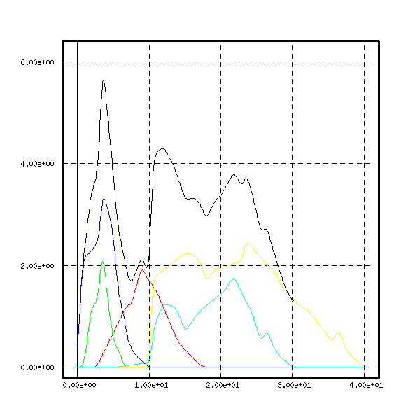
In figure 12 we represent the 21 curves for $a=0$ to $10$. The curve for $a=0$ is on the top, the one for $a=0.5$ just below, and so on. The curve for $a=0$ is a good approximation for the exponential.

3.4 Use of numerical data

Program example_load, file demo.cmd

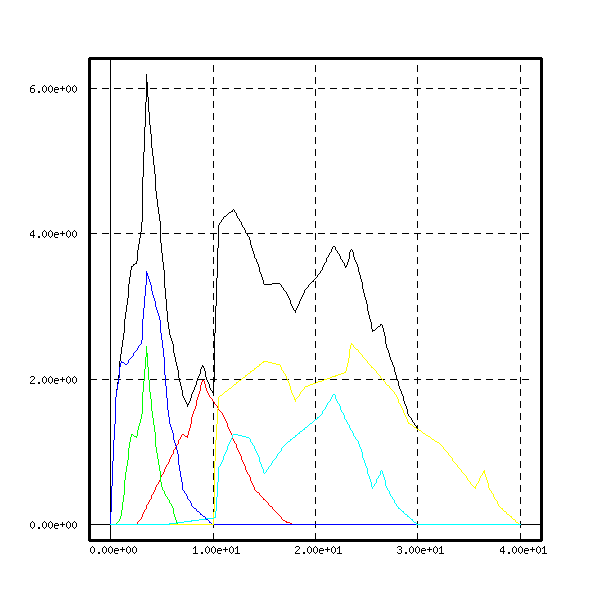
In this program file we use 5 real functions defined by data files contained in the directory bin/res/data/. We load the 5 functions, find the smallest interval which contains all the intervals where the functions are defined, and compute the sum of the 5 functions on this big interval.

Then we smooth the 5 functions and their sum by making convolutions with the function

$$\sqrt{\frac{8}{\pi}}e^{-8x^2}$$

To run the program, when demo.cmd is loaded, type the commands :

 - funct -> clear X
 - funct -> example_load

:example_load
1
1
-1
Max=0.
Min=0.
;
; the 5 functions are loaded and created (f1 to f5)
do i 1 5
load_create_f x!(i) f!(i) data/data!(i)
desc_func f!(i)
if< xmax-Max zz
Max=xmax
zz:
if> xmin-Min yy
Min=xmin
yy:
enddo
;
;
; the function that will contain the sum is created
xrange_f xr 1 1001
fix_xrange_f xr Min (Max-Min)/1000.
function_f f xr
;
;
; the sum is computed
do i 1 5
add_func f f!(i) f
enddo
;
min_func f
max_func f
;
defframe ff
frame ff  Min-2.  Max+2.  fmin_func-.2  fmax_func+.2  10. 2.
;
; graphics
draw_graph_ex_load X f
;
;
; smooth versions of the functions
;
xrange_f xrb 1 2001
fix_xrange_f xrb Min-5 (Max+10-Min)/2000.
xrange_f xw 1 201
fix_xrange_f xw -1. 0.01
function_f liss xw
a=sqrt(pi)/sqrt(8)
fill_func liss exp(-8*x*x)/a
function_f FF xrb

do i 1 5
function_f F!(i) xrb
function_f FF!(i) xrb
copy_func f!(i) F!(i)
convol F!(i) liss FF!(i) 256
add_func FF FF!(i) FF
enddo
draw_graph_ex_load X FF
;
;
destroy x1
destroy x2
destroy x3
destroy x4
destroy x5
destroy xr
destroy xrb
destroy xw
destroy ff
;
;
:draw_graph_ex_load
3
0
-1
setframe #1 ff
funct_plot #2 #1 ff Min Max 1000
setcolor #1 red
funct_plot #(2)1 #1 ff Min Max 1000
setcolor #1 green
funct_plot #(2)2 #1 ff Min Max 1000
setcolor #1 blue
funct_plot #(2)3 #1 ff Min Max 1000
setcolor #1 yellow
funct_plot #(2)4 #1 ff Min Max 1000
setcolor #1 Lblue
funct_plot #(2)5 #1 ff Min Max 1000
;
;
:clean_ex_load
1
0
-1
destroy XX
destroy x1
destroy x2
destroy x3
destroy x4
destroy x5
destroy xr
destroy ff
;

Here are represented the 5 functions and their sum, which is the function on the top, since the 5 functions were positive.

The smooth versions of the functions is represented below

3.5 Convolution of functions

Program convol1, file demo.cmd

This program computes the convolution of the function

$$f(x) \ = \ e^{-8x^2}$$

with itself. The result should be

$$g(x) \ = \ \frac{\sqrt{\pi}}{4}e^{-4x^2}$$

We compute $f*f$ and $g$ and compare them.

To run the program, when demo.cmd is loaded, type the commands :

 - funct -> clear X
 - funct -> convol1

:convol1
1
0
-1
xrange_f xr 1 401   
fix_xrange_f xr -2 .01
xrange_f xr2 1 401
fix_xrange_f xr2 -2 .01
xrange_f xr3 1 1001
fix_xrange_f xr3 -5 .01
function_f f xr
function_f f2 xr2
function_f f3 xr3
fill_func f exp(-8*x*x)
fill_func f2 exp(-8*x*x)
convol f f2 f3 1024
function_f f4 xr3
a=sqrt(pi)/4
fill_func f4 a*exp(-4.*x*x)
defframe ff
frame ff -1.5 1.5 -.1 0.5 2 .2
setframe X ff
setcolor X red
funct_plot f3 X ff -1.5 1.5 1000
setcolor X blue
funct_plot f4 X ff -1.5 1.5 1000
destroy xr
destroy xr2
destroy xr3
destroy ff
;

The two functions are shown on figure 15.

3.6 Fourier transform and FFT

Program fft4, file demo.cmd

In this program we compute the Fourier transform of the complex function

$$f(x) \ = \ 2e^{-8x^2}\sin(5(0.2-x)) \ + \ i.\log(1+x^2)\sin(1.5-x)$$

defined on the interval $[0,1]$. We then compute the FFT of this function on 1024 points. Finally we want to obtain a more precise FFT of $f(x)$. For this we build a new function defined on $[0,2]$, equal to $f(x)$ on $[0,1]$ and which vanishes on $[1,2]$, and compute the FFT of this new function on 2048 points.

To run the program, when demo.cmd is loaded, type the commands :

 - funct -> clear X
 - funct -> fft4

:fft4
1
0
-1
xrange_f xr 1 201
fix_xrange_f xr -1 0.01
function_f fr xr
fill_func fr 2.*exp(-8*x*x)*sin((.2-x)*5.)
function_f fi xr
fill_func fi log(1+x*x)*sin(1.5-x)
function_fC f xr
imag_fix fi f
real_fix fr f
defframe ff0
frame ff0 -1 1 -.6 2. .25 .2
setframe X ff0
setcolor X red
funct_plot fr X ff0 -1 1 1000
setcolor X blue
funct_plot fi X ff0 -1 1 1000
def_four Tr f 1024
xrange_f X2 1 1000
fix_xrange_f X2 -25 .05
function_fC F X2
function_fC F2 X2
trans_four Tr F
fft f F2 1024
xrange_f xrb 1 401
fix_xrange_f xrb -1 0.01
fix_func_C f 201 0 0
function_fC fb xrb
copy_func f fb
function_fC F2b X2
fft fb F2b 2048
color_echo green
echo Hit Enter\n
color_echo black
waitkey
clear X
defframe ff
frame ff -25 25 -0.6 0.6 10 .2
setframe X ff
setcolor X red
funct_plot F X ff -25 25 1000
setcolor X green
funct_plot F2 X ff -25 25 1000
setcolor X blue
funct_plot F2b X ff -25 25 1000
function_f F2.i X2
imag F2 F2.i
function_f F.i X2
imag F F.i
echo Here the red curve is the real part of the Fourier transform of f(x),\n
echo the green curve is the real part of the FFT on 1024 points, and the blue\n
echo one is the real part of the FFT on 2048 points.\n
color_echo green
echo Hit Enter\n
color_echo black
waitkey
clear X
setframe X ff
setcolor X green
funct_plot F2.i  X ff -25 25 1000
setcolor X red
funct_plot F.i  X ff -25 25 1000
setcolor X blue
function_f F2b.i X2
imag F2b F2b.i
funct_plot F2b.i  X ff -25 25 1000
echo Here the red curve is the imaginary part of the Fourier transform of f(x),\n
echo the green curve is the imaginary part of the FFT on 1024 points, and the blue\n
echo one is the imaginary part of the FFT on 2048 points.\n
;
;
destroy xr
destroy xrb
destroy X2
destroy ff
destroy Tr
destroy ff0
;

The real and imaginary parts of the function $f(x)$ are represented here

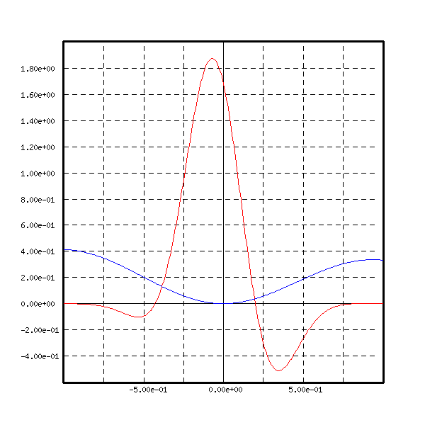
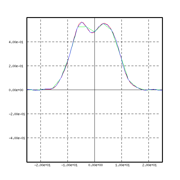
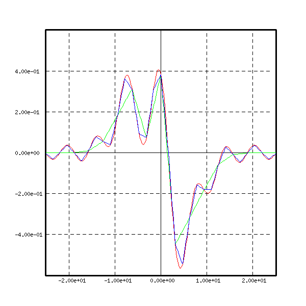
The real and imaginary parts of the Fourier transform of $f$ are the red curves on the next 2 figures
The real and imaginary parts of the first FFT of $f$ are the green curves.
The real and imaginary parts of the second FFT of $f$ are the blue curves.

3.7 Iteration of functions

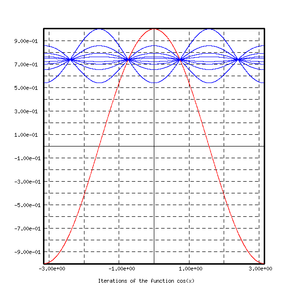
Program Fix_point, file demo.cmd

In this program we compute successive compositions of the function $cos(x)$ : $cos(x)$, $cos(cos(x))$, $cos(cos(cos(x)))$, ... The limit should be the constant function $f(x)=c$ where $c$ is the root of the equation $cos(x)=x$.

To run the program, when demo.cmd is loaded, type the commands :

 - funct -> clear X
 - funct -> Fix_point

:Fix_point
1
0
-1
;
xrange xr 1 4001
fix_xrange xr -pi pi/2000
function f xr
function g xr
fill_func f cos(x)
defframe F
frame F -pi pi -1 1 1 0.1 2 2
setframe X F
title X F Iterations of the function cos(x)
setcolor X red 
funct_plot f X F -pi pi 4000
function g xr
comp_func f f g
setcolor X blue             
funct_plot g X F -pi pi 4000
comp_func f g g             
funct_plot g X F -pi pi 4000
comp_func f g g             
funct_plot g X F -pi pi 4000
comp_func f g g             
funct_plot g X F -pi pi 4000
comp_func f g g             
funct_plot g X F -pi pi 4000
comp_func f g g             
funct_plot g X F -pi pi 4000
comp_func f g g             
funct_plot g X F -pi pi 4000
comp_func f g g             
funct_plot g X F -pi pi 4000
destroy xr
destroy F
;

The function $cos(x)$ and several iterated functions are represented here