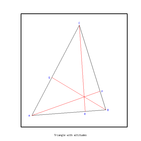
Program ex0, file geom.cmd
In this program we draw a triangle and its altitudes. We do the following steps :
To run the program, when geom.cmd is loaded, type the commands :
 - funct -> clear X
 - funct -> ex0
:ex0
1
0
-1
;
;
defframe f
frame f 0 1 0 1 1 1
setframe X f
setcolor X black
title X f Triangle with altitudes
point A
point B
point C
coord A 0.1 0.1
coord B 0.8 0.15
coord C 0.55 0.9
draw A X f
draw_to B X f
draw_to C X f
draw_to A X f
line AB
line BC
line CA
span_l AB A B
span_l BC B C
span_l CA C A
point HA
point HB
point HC
orthoproj A BC HA
orthoproj B CA HB
orthoproj C AB HC
draw A X f
setcolor X blue
putstring X f -O A
setcolor X red
draw_to HA X f
setcolor X blue
putstring X f -E P
draw B X f
setcolor X blue
putstring X f -E B
setcolor X red
draw_to HB X f
setcolor X blue
putstring X f -O Q
draw C X f
setcolor X blue
putstring X f -N C
setcolor X red
draw_to HC X f
setcolor X blue
putstring X f -S R
destroy A
destroy B
destroy C
destroy AB
destroy BC
destroy CA
destroy HA
destroy HB
destroy HC
destroy f
The triangle and its altitudes are represented here
Program ex1, file geom.cmd
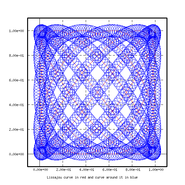
This program requires 3 arguments : the first ![]() and
the second
and
the second ![]() will define the Lissajou curve : it is
given by the parametric equations
will define the Lissajou curve : it is
given by the parametric equations
 - funct -> clear X
 - funct -> ex1 5 6 800
:ex1
4
0
-1
n=#1
if> n-#2 E1
n=#2
E1:
n0=n
if> n-#3 E2
n=#3
E2:
n=n*40
n0=n0*100
dx=2*pi/n0
xrange xr 1 n0+1
fix_xrange xr 0 dx
function xx xr
function yy xr
fill_func xx 0.5+0.5*cos(#1*x)
fill_func yy 0.5+0.5*sin(#2*x)
defframe f
frame f -0.1 1.1 -0.1 1.1 0.2 0.2
setframe X f
setcolor X black
title X f Lissajou curve in red and curve around it in blue
setcolor X red
polyg p 10
polyg_funct p xx yy
draw p X f
xrange xr2 1 n
dx=2*pi/n
fix_xrange xr2 0 dx
function xx2 xr2
function yy2 xr2
fill_func xx2 0.5+0.5*cos(#1*x)+0.05*cos(#3*x)
fill_func yy2 0.5+0.5*sin(#2*x)+0.05*sin(#3*x)
setcolor X blue
polyg q 10
polyg_funct q xx2 yy2
draw q X f
clean_ex1
;
;
:clean_ex1
1
1
-1
destroy xr
destroy xr2
destroy p
destroy q
destroy f
The Lissajou curve and the curve around it are represented here
Program ex5b, file geom.cmd
This program draws a moving triangle. One argument a is required : the program will successively draw and erase 400*a triangles.
To run the program, when geom.cmd is loaded, type the commands :
 - funct -> clear X
 - funct -> ex5b 1
:ex5b
2
0
-1
ex3
clear X
setframe X f noax
setcolor X black
title X f Moving triangle with altitudes, medians and bissectrices
do j 1 #1
do i 0 400
coord A -5/7+i/70 -3/11+i/55
coord B -2/3+i/60 6-i/80
coord C 25/3-i/75 -17/26+i/65
progb
xflush
sleep 10
clean_progb
enddo
do i 0 400
coord A 5-i/70 7-i/55
coord B 6-i/60 1+i/80
coord C 3+i/75 5.5-i/65
progb
xflush
sleep 10
clean_progb
enddo
enddo
progb
destroy f
destroy A
destroy B
destroy C
destroy CC
destroy AB
destroy BC
destroy AC
destroy AA
destroy BB
destroy lA
destroy lB
destroy lC
destroy mA
destroy mB
destroy mC
destroy MA
destroy MB
destroy MC
;
;
:progb
1
0
-1
setcolor X black
span_l AB A B
span_l AC A C
bissec AB AC lA
draw A X f
draw_to B X f
draw A X f
draw_to C X f
setcolor X red
span_l BC B C
inters lA BC AA
draw A X f
draw_to AA X f
draw B X f
inverse AB AB
setcolor X black
draw_to C X f
bissec AB BC lB
inters lB AC BB
setcolor X red
draw B X f
draw_to BB X f
bissec AC BC lC
inters lC AB CC
draw C X f
draw_to CC X f
middle A B mC
middle C B mA
middle A C mB
orthoproj A BC MA
orthoproj B AC MB
orthoproj C AB MC
setcolor X green
draw A X f
draw_to mA X f
draw B X f
draw_to mB X f
draw C X f
draw_to mC X f
setcolor X blue
draw A X f
draw_to MA X f
draw B X f
draw_to MB X f
draw C X f
draw_to MC X f
;
;
:clean_progb
1
0
-1
setcolor X white
draw A X f
draw_to B X f
draw A X f
draw_to C X f
draw A X f
draw_to AA X f
draw B X f
draw_to C X f
draw B X f
draw_to BB X f
draw C X f
draw_to CC X f
draw A X f
draw_to mA X f
draw B X f
draw_to mB X f
draw C X f
draw_to mC X f
draw A X f
draw_to MA X f
draw B X f
draw_to MB X f
draw C X f
draw_to MC X f
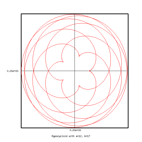
Program ex4, file geom.cmd
This program defines and draws curves called hypocycloids.
They are
defined by the parametric equations :
To run the program, when geom.cmd is loaded, type the commands :
 - funct -> clear X
 - funct -> ex4 12 17
:ex4
3
0
-1
xrange xr 1 10000
fix_xrange xr 0 2*pi/300
function xx xr
function yy xr
a=#1
b=#2
c=a-b
d=a/b-1
fill_func xx c*cos(x)+b*cos(d*x)
fill_func yy c*sin(x)-b*sin(d*x)
defframe f
frame f -abs(c)-b abs(c)+b -abs(c)-b abs(c)+b abs(c)+b abs(c)+b
setframe X f
setcolor X black
title X f Hypocycloid with a=12, b=17
setcolor X red
polyg p 10
polyg_funct p xx yy
draw p X f
destroy xr
destroy p
destroy f
The hypocycloid with ![]() and
and ![]() is
represented below
is
represented below
Program ex1c, file geom.cmd
This programs defines two Lissajou curves with parametric
coordinates
 - funct -> clear X
 - funct -> ex1c 3 4 7 8 200
:ex1c
5
0
-1
n=#1
if> n-#2 E1
n=#2
E1:
if> n-#3 E2
n=#3
E2:
if> n-#4 E3
n=#4
E3:
n=30*n
dx=2*pi/n
xrange xr 1 n+10
fix_xrange xr -dx-dx dx
function xx xr
function yy xr
clear X
defframe f
frame f -0.1 1.1 -0.1 1.1 2 2
setframe X f noax
setcolor X black
title X f Curves between two Lissajou curves
polyg p 10
do i 0 #5
t=i/#5
u=1-t
fill_func xx 0.5+0.5*(t*cos(#1*x)+u*cos(#3*x))
fill_func yy 0.5+0.5*(t*sin(#2*x)+u*sin(#4*x))
polyg_funct p xx yy
setcolor X red
draw p X f
xflush
sleep 20
setcolor X white
draw p X f
enddo
setcolor X black
setcolor X red
draw p X f
setcolor X black
destroy xr
destroy f
destroy p
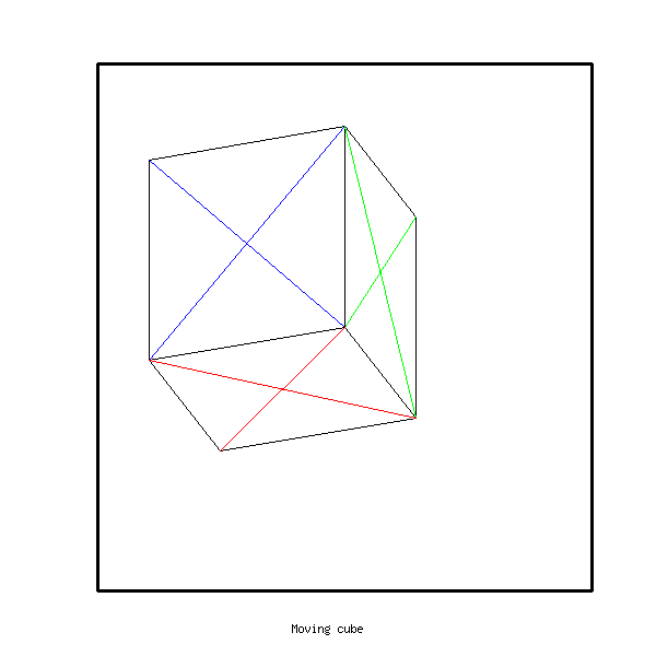
Program ex6d, file geom.cmd
This programs draws a moving cube. It needs one argument : the number of sucessive cubes that will be drawn and erased. To run the program, when geom.cmd is loaded, type the commands :
 - funct -> clear X
 - funct -> ex6d 2123
:ex6d
2
0
-1
point O
point A
point B
point C
point O2
point A2
point B2
point C2
vector OB
vector BA2
vector AA2
vector A2O2
vector BB2
vector B2O2
vector B2C
vector CC2
vector OC
defframe f
frame f -0.8 0.8 -0.8 0.8 3 3
setcolor X black
title X f Moving cube
coord O -3 0
setframe X f noax
draw O X f
coord O 3 0
setcolor X white
draw_to O X f
coord O 0 -3
draw O X f
coord O 0 3
draw_to O X f
vector U
vector V
vector Tr
dt=pi/400
do i 1 #1
t=i*dt
som_pard t 2*t 3*t abs(cos(t/4))
transl cos(5*t)/2 sin(4*t)/2
somm
drawubec
setframe X f noax
sleep 10
xflush
clean_cubec
enddo
drawubec
destroy O
destroy A
destroy B
destroy C
destroy O2
destroy A2
destroy B2
destroy C2
destroy f
destroy OB
destroy BA2
destroy AA2
destroy A2O2
destroy BB2
destroy B2O2
destroy B2C
destroy CC2
destroy OC
destroy U
destroy V
destroy Tr
;
;
:som_pard
5
0
-1
; 1 : theta0, 2 : phi0, 3 : rot
c0=cos(#1)
s0=sin(#1)
sp0=sin(#2)
cp0=cos(#2)
cr=cos(#3)
sr=sin(#3)
coord A #4*c0*cp0 #4*s0*cp0
coord B #4*(-s0*cr+sp0*c0*sr) #4*(c0*cr+sp0*s0*sr)
coord C #4*(s0*sr+sp0*c0*cr) #4*(-c0*sr+sp0*s0*cr)
;
;
:drawubec
1
0
-1
vect_s
; face O B A2 A
ext_prod OB BA2
if< ext_p XXX1
setcolor X black
draw_sqr O B A2 A
setcolor X blue
draw_diag O B A2 A
; face A A2 O2 C2
XXX1:
ext_prod AA2 A2O2
if< ext_p XXX2
setcolor X black
draw_sqr A A2 O2 C2
setcolor X green
draw_diag A A2 O2 C2
; face B B2 O2 A2
XXX2:
ext_prod BB2 B2O2
if< ext_p XXX3
setcolor X black
draw_sqr B B2 O2 A2
setcolor X red
draw_diag B B2 O2 A2
; face B2 C C2 O2
XXX3:
ext_prod B2C CC2
if< ext_p XXX4
setcolor X black
draw_sqr B2 C C2 O2
setcolor X blue
draw_diag B2 C C2 O2
; face B O C B2
XXX4:
ext_prod OB OC
if> ext_p XXX5
setcolor X black
draw_sqr B O C B2
setcolor X green
draw_diag B O C B2
; face C2 C O A
XXX5:
ext_prod CC2 OC
if< ext_p XXX6
setcolor X black
draw_sqr C2 C O A
setcolor X red
draw_diag C2 C O A
;
XXX6:
;
;
:clean_cubec
1
0
-1
setcolor X white
vect_s
; face O B A2 A
ext_prod OB BA2
if< ext_p XXX1
draw_sqr O B A2 A
draw_diag O B A2 A
; face A A2 O2 C2
XXX1:
ext_prod AA2 A2O2
if< ext_p XXX2
draw_sqr A A2 O2 C2
draw_diag A A2 O2 C2
; face B B2 O2 A2
XXX2:
ext_prod BB2 B2O2
if< ext_p XXX3
draw_sqr B B2 O2 A2
draw_diag B B2 O2 A2
; face B2 C C2 O2
XXX3:
ext_prod B2C CC2
if< ext_p XXX4
draw_sqr B2 C C2 O2
draw_diag B2 C C2 O2
; face B O C B2
XXX4:
ext_prod OB OC
if> ext_p XXX5
draw_sqr B O C B2
draw_diag B O C B2
; face C2 C O A
XXX5:
ext_prod CC2 OC
if< ext_p XXX6
draw_sqr C2 C O A
draw_diag C2 C O A
;
XXX6:
;
;
:draw_diag
5
0
-1
draw #1 tt f
draw_to #3 tt f
draw #2 tt f
draw_to #4 tt f
;
;
:somm
1
0
-1
; U=vec(OC), V=vec(OB)
vector_p O C U
vector_p O B V
point_v A U C2
point_v B U B2
point_v A V A2
point_v A2 U O2
;
;
:vect_s
1
0
-1
vector_p O B OB
vector_p B A2 BA2
vector_p A A2 AA2
vector_p A2 O2 A2O2
vector_p B B2 BB2
vector_p B2 O2 B2O2
vector_p B2 C B2C
vector_p C C2 CC2
vector_p O C OC
;
;
:draw_sqr
5
0
-1
draw #1 tt f
draw_to #2 tt f
draw_to #3 tt f
draw_to #4 tt f
draw_to #1 tt f
;
One of these cubes is shown here
Program ex7, file geom.cmd
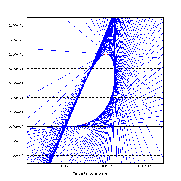
This program defines a curve with parametric coordinates
 - funct -> clear X
 - funct -> ex7 100
:ex7
2
0
-1
xrange xr 1 1000
fix_xrange xr 0 0.001
function xx xr
function yy xr
fill_func xx x*(1-x)
fill_func yy sin(pi*x*x)
defframe f
frame f -0.2 0.5 -0.5 1.5 0.2 0.2
setframe X f
setcolor X black
title X f Tangents to a curve
setcolor X red
polyg p 10
polyg_funct p xx yy
draw p X f
polyg_curv p p 1035
length_pol p
dt=length_pol/#1
line L
setcolor X blue
do i 1 #1
x=i*dt
tangent_p p x L
draw L X f
enddo
destroy xr
destroy f
destroy p
destroy L
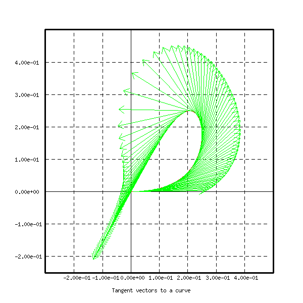
The curve and its tangent lines are shown on the first figure. The
program ex7b
is analogous, but draws tangent vectors instead of tangent lines. The
curve
and 100 tangent vectors are shown on the next figure.
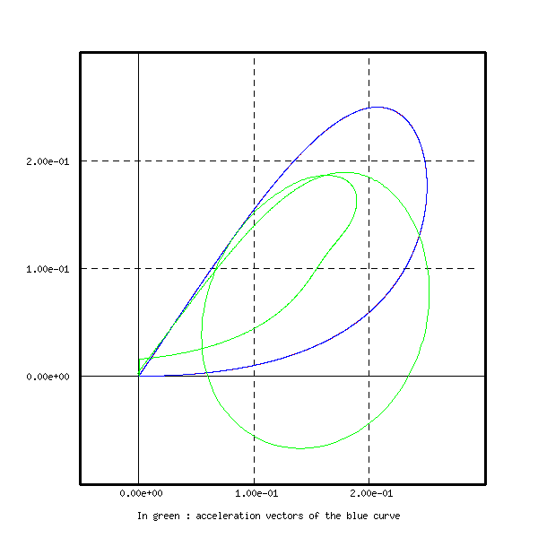
Program ex7c, file geom.cmd
To run the program, when geom.cmd is loaded, type the commands :
This program defines a curve with parametric coordinates
To run the program, when geom.cmd is loaded, type the commands :
 - funct -> clear X
 - funct -> ex7c 1000
:ex7c
2
0
-1
xrange xr 1 5000
fix_xrange xr 0 0.0002
function xx xr
function yy xr
fill_func xx x*(1-x)
fill_func yy 0.25*sin(pi*x*x)
defframe f
frame f -0.05 0.3 -0.1 0.3. 0.1 0.1
setframe X f
setcolor X black
title X f In green : acceleration vectors of the blue curve
setcolor X red
polyg p 10
polyg_funct p xx yy
draw p X f
polyg q 10
polyg_curv p q 2000
setcolor X blue
length_pol q
draw q X f
dt=length_pol/#1
line L
vector v
point A
point B
point B0
setcolor X green
do i 1 #1-1
x=i*dt
accel_p q x v A
multiply v 0.01 v
point_v A v B
draw_to B X f
enddo
destroy xr
destroy f
destroy A
destroy B0
destroy B
destroy p
destroy q
destroy L
destroy v
;
The initial curve and the curve of acceleration vectors are
represented here
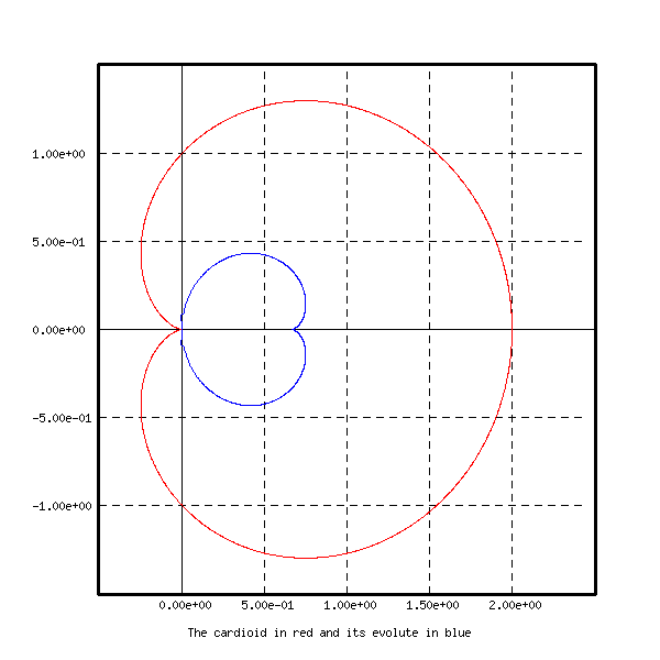
Program evolx2, file geom.cmd
This program defines a curve, called cardioid, with
parametric
coordinates
 - funct -> clear X
 - funct -> evolx2
:evolx2
1
0
-1
xrange xr 1 4000
fix_xrange xr 0 pi/1900
function xx xr
function yy xr
fill_func xx (1+cos(x))*cos(x)
fill_func yy (1+cos(x))*sin(x)
defframe f
frame f -0.5 2.5 -1.5 1.5 0.5 0.5
setframe X f
setcolor X black
title X f The cardioid in red and its evolute in blue
setcolor X red
polyg p 10
polyg_funct p xx yy
polyg q 10
polyg_curv p q 2000
draw q X f
polyg r 10
setcolor X blue
evol q r
draw r X f 0 1900
destroy xr
destroy f
destroy p
destroy q
destroy r
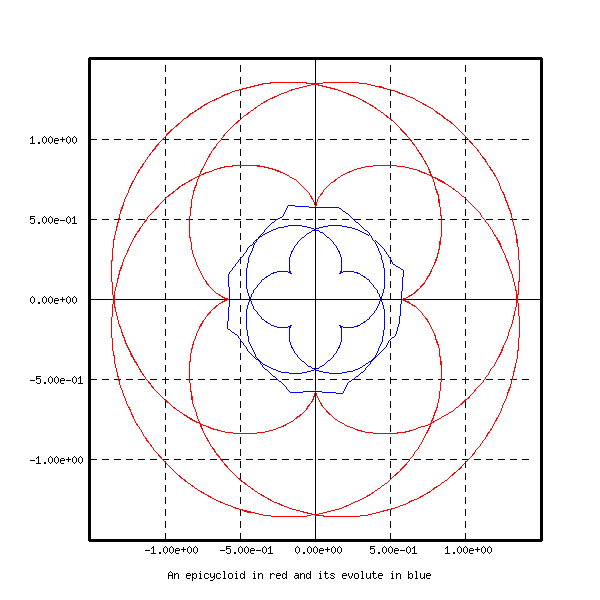
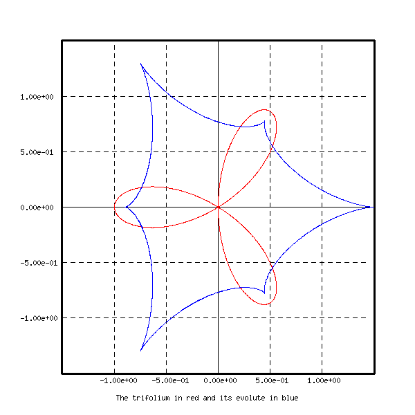
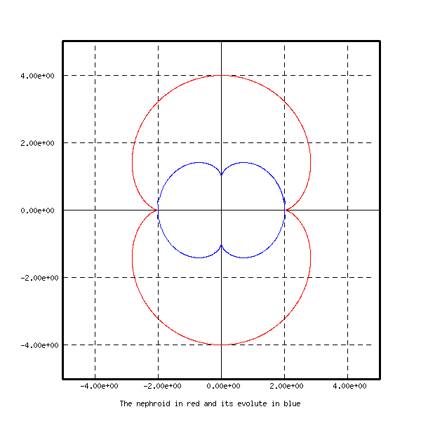
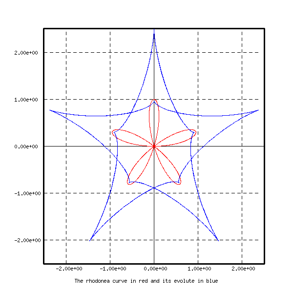
The cardioid and its evolute are shown on the first figure below.
The programs evolx3,
evolx4, evolx5, evolx6, evolx7
are analogous, and
draw respectively an epicycloid, a trifolium, a nephroid,
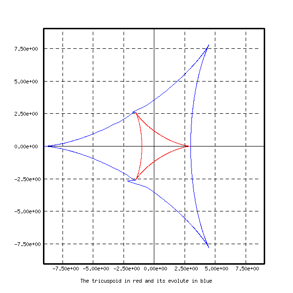
a Rhodonea curve and a tricuspoid with their
evolutes. These curves are represented on the next figures.
Program ex9, file geom.cmd
This program computes a geometric locus associated to a triangle.
Let ![]() be a triangle,
be a triangle, ![]() a
real number and
a
real number and
The program ex9 draws the rectangle ![]() ,
where
,
where ![]() ,
, ![]() and
and ![]() , where
, where ![]() is a real number.
It computes then the point
is a real number.
It computes then the point ![]() for many values of
for many values of ![]() , joining two sucessive points. We obtain
a curve that seems to be asymptotic to a line when
, joining two sucessive points. We obtain
a curve that seems to be asymptotic to a line when ![]() , and to
have a node. The reader may try to prove this by direct computations.
, and to
have a node. The reader may try to prove this by direct computations.
The program needs an argument, which is the first coordinate ![]() of
of ![]() .
To run the program, when geom.cmd is loaded, type the
commands :
.
To run the program, when geom.cmd is loaded, type the
commands :
 - funct -> clear X
 - funct -> ex9 0.85
:ex9
2
0
-1
point A
coord A 0 0
point B
coord B 1 0
point C
coord C #1 0.8660254037844386
line AB
span_l AB A B
line BC
span_l BC B C
line AC
span_l AC A C
defframe f
frame f -0.1 1.5 -0.1 1.5 0.5 0.5
setframe X f
setcolor X black
title X f A triangle and a geometric locus associated to it
draw A X f
putstring X f -SO A
draw B X f
putstring X f -SE B
draw C X f
putstring X f -N C
setcolor X red
draw B X f
draw_to C X f
draw_to A X f
draw_to B X f
point AT
point BT
point CT
point XT
vector ct
vector xt
vector bt
vector V
vector W
vector X
setcolor X blue
do i -1250 650 4
t=i/100
bary2 A B t AT
bary2 B C t BT
bary2 C A t CT
dist AT BT
ct=dist_p
dist CT BT
at=dist_p
dist AT CT
bt=dist_p
vector_p AT BT ct
vector_p AT CT bt
multiply ct bt/(at+bt+ct) V
multiply bt ct/(at+bt+ct) W
add V W X
point_v AT X XT
if> i+1250 XXX
draw XT X f
XXX:
draw_to XT X f
enddo
destroy A
destroy B
destroy C
destroy AB
destroy BC
destroy AC
destroy AT
destroy BT
destroy CT
destroy XT
destroy ct
destroy xt
destroy bt
destroy V
destroy W
destroy X
destroy f
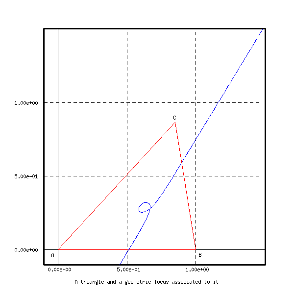
The triangle ![]() and the geometric locus of points
and the geometric locus of points ![]() (the blue curve) are
represented below
(the blue curve) are
represented below
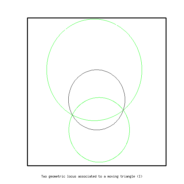
Program ex16, file geom.cmd
In this program we consider a circle with two fixed points on it. A third point is moving on the circle and defines a triangle with the two fixed points. We are interested by the following two geometric locus :
To run the program, when geom.cmd is loaded, type the commands :
 - funct -> clear X
 - funct -> ex16
:ex16
1
0
-1
defframe f
frame f 0 1 0 1 1 1
setframe X f noax
setcolor X black
title X f Two geometric locus associated to a moving triangle (I)
circle C00
point O
coord O 0.5 0.5
coord C00 O 0.45
point A
point B
point C
point P
point P1
line BA
line AB
line BC
line AC
line lA
line lB
line lC
line lA1
line lB1
line lC1
point A0
point B0
point C0
point A1
point B1
point C1
polyg Pol 361
polyg Pol2 361
ang1=-20
ang2=210
da=pi/180
coord A 0.5+0.45*cos(ang1*da) 0.5+0.45*sin(ang1*da)
coord B 0.5+0.45*cos(ang2*da) 0.5+0.45*sin(ang2*da)
span_l AB A B
span_l BA B A
j=-1
;
do i ang1+1 ang1+361
ang=i*da
j=j+1
coord C 0.5+0.45*cos(ang) 0.5+0.45*sin(ang)
span_l BC B C
span_l AC A C
bissec AB AC lA
bissec BA BC lB
bissec AC BC lC
inters BC lA A0
inters AB lC C0
inters AC lB B0
inters lA lB P
middle A B C1
middle B C A1
middle A C B1
span_l lA1 A A1
span_l lB1 B B1
span_l lC1 C C1
inters lA1 lB1 P1
show P
coord Pol j point_x point_y
show P1
coord Pol2 j point_x point_y
draw C00 X f
setcolor X red
draw A X f
draw_to B X f
draw_to C X f
draw_to A X f
setcolor X violet
draw C X f
draw_to C0 X f
draw A X f
draw_to A0 X f
draw B X f
draw_to B0 X f
setcolor X blue
draw C X f
draw_to C1 X f
draw A X f
draw_to A1 X f
draw B X f
draw_to B1 X f
;
sleep 10
setcolor X white
draw A X f
draw_to B X f
draw_to C X f
draw_to A X f
draw C X f
draw_to C0 X f
draw A X f
draw_to A0 X f
draw B X f
draw_to B0 X f
draw C X f
draw_to C1 X f
draw A X f
draw_to A1 X f
draw B X f
draw_to B1 X f
;
setcolor X green
draw Pol X f 0 j
setcolor X blue
draw Pol2 X f 0 j
setcolor X black
enddo
draw C00 X f
destroy f
destroy O
destroy A
destroy B
destroy C
destroy P
destroy P1
destroy A0
destroy B0
destroy C0
destroy A1
destroy B1
destroy C1
destroy BA
destroy AB
destroy BC
destroy AC
destroy lA
destroy lB
destroy lC
destroy lA1
destroy lB1
destroy lC1
destroy C00
destroy Pol
destroy Pol2
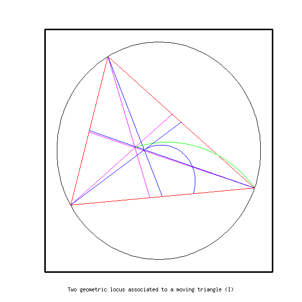
The locus of the intersections of medians is the blue curve, and the
locus of
the intersections of bissectrices is the green one. The final result is
shown on the second figure below. An intermediate result is represented
on the first figure.
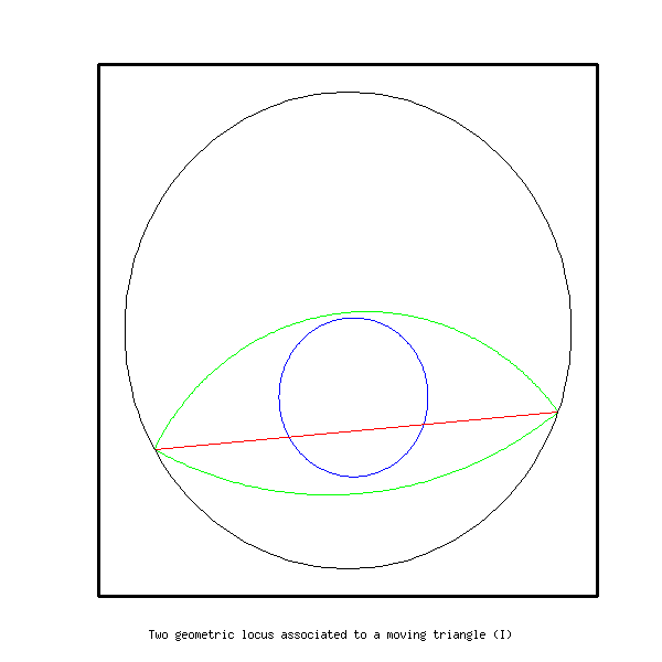
The blue curve seems to be a circle, it is not very hard to prove that
it is
actually a circle, of radius ![]() of the radius of the initial
circle.
of the radius of the initial
circle.
The green circles seem to be arc of circles, are they are actually,
but this is
a little less easy to prove. To obtain two complete green circles it is
necessary to consider also the exterior bissectrices (cf. 4.12).
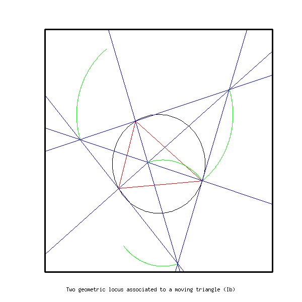
Program ex16c, file geom.cmd
In this program we consider a circle with two fixed points on it. A third point is moving on the circle and defines a triangle with the two fixed points. We are interested by the locus of the intersections of the interior and exterior bissectrices.
It can be proved that these intersections points go over two circles
that
contain the two fixed points ![]() ,
, ![]() . The centers of
the two circles are
the points of the initial circle that are on the diameter which is
perpendicular to
. The centers of
the two circles are
the points of the initial circle that are on the diameter which is
perpendicular to ![]() .
.
The program draws a sequence of triangles with their bissectrices. The intersections points are put in two polygons. Each time a new triangle is drawn, a vertex of each polygon is added.
The circle has center (0.5,0.5) and radius 0.45. The first point on
the circle has angle 20 (in degrees), i.e its coordinates are ![]() , with
, with ![]() .
The program needs an argument, it is the angle of the second point.
To run the program, when geom.cmd is loaded, type the
commands :
.
The program needs an argument, it is the angle of the second point.
To run the program, when geom.cmd is loaded, type the
commands :
 - funct -> clear X
 - funct -> ex16c 210
:ex16c
2
0
-1
defframe f
frame f -0.6 1.6 -0.48 1.72 5 5
setframe X f noax
setcolor X black
title X f Two geometric locus associated to a moving triangle (Ib)
circle C00
point O
coord O 0.5 0.5
coord C00 O 0.45
point A
point B
point C
point P
point PA
point PB
point PC
line BA
line AB
line BC
line AC
line CA
line lA
line lB
line lC
line lA2
line lB2
line lC2
polyg Pol 361
polyg Pol2 361
polyg Pol3 361
polyg Pol4 361
polyg Polb 361
polyg Pol2b 361
polyg Pol3b 361
polyg Pol4b 361
ang1=-20
ang2=#1
da=pi/180
coord A 0.5+0.45*cos(ang1*da) 0.5+0.45*sin(ang1*da)
coord B 0.5+0.45*cos(ang2*da) 0.5+0.45*sin(ang2*da)
span_l AB A B
span_l BA B A
j=-1
;
do i ang1+1 ang2-1
ang=i*da
j=j+1
j0=j
coord C 0.5+0.45*cos(ang) 0.5+0.45*sin(ang)
span_l BC B C
span_l AC A C
span_l CA C A
bissec AB AC lA
bissec BA BC lB
bissec AC BC lC
bissec AB BC lB2
bissec AC BA lA2
bissec CA BC lC2
inters lA lB P
inters lC2 lA2 PB
inters lC2 lB2 PA
inters lA2 lB2 PC
show P
coord Pol j point_x point_y
show PA
coord Pol2 j point_x point_y
show PB
coord Pol3 j point_x point_y
show PC
coord Pol4 j point_x point_y
draw C00 X f
setcolor X red
draw A X f
draw_to B X f
draw_to C X f
draw_to A X f
setcolor X blue
draw lA X f
draw lA2 X f
draw lB X f
draw lB2 X f
draw lC X f
draw lC2 X f
;
sleep 10
setcolor X white
draw A X f
draw_to B X f
draw_to C X f
draw_to A X f
draw lA X f
draw lA2 X f
draw lB X f
draw lB2 X f
draw lC X f
draw lC2 X f
;
setcolor X green
draw Pol X f 0 j
draw Pol2 X f 0 j
draw Pol3 X f 0 j
draw Pol4 X f 0 j
setcolor X black
setframe X f noax
enddo
;
j=-1
do i ang2+1 ang1+359
ang=i*da
j=j+1
coord C 0.5+0.45*cos(ang) 0.5+0.45*sin(ang)
span_l BC B C
span_l AC A C
span_l CA C A
bissec AB AC lA
bissec BA BC lB
bissec AC BC lC
bissec AB BC lB2
bissec AC BA lA2
bissec CA BC lC2
inters lA lB P
inters lC2 lA2 PB
inters lC2 lB2 PA
inters lA2 lB2 PC
show P
coord Polb j point_x point_y
show PA
coord Pol2b j point_x point_y
show PB
coord Pol3b j point_x point_y
show PC
coord Pol4b j point_x point_y
draw C00 X f
setcolor X red
draw A X f
draw_to B X f
draw_to C X f
draw_to A X f
setcolor X blue
draw lA X f
draw lA2 X f
draw lB X f
draw lB2 X f
draw lC X f
draw lC2 X f
;
sleep 10
setcolor X white
draw A X f
draw_to B X f
draw_to C X f
draw_to A X f
draw lA X f
draw lA2 X f
draw lB X f
draw lB2 X f
draw lC X f
draw lC2 X f
;
setcolor X green
draw Polb X f 0 j
draw Pol2b X f 0 j
draw Pol3b X f 0 j
draw Pol4b X f 0 j
draw Pol X f 0 j0
draw Pol2 X f 0 j0
draw Pol3 X f 0 j0
draw Pol4 X f 0 j0
setcolor X black
setframe X f noax
enddo
draw C00 X f
destroy f
destroy O
destroy A
destroy B
destroy C
destroy P
destroy PA
destroy PB
destroy PC
destroy BA
destroy AB
destroy BC
destroy AC
destroy CA
destroy lA
destroy lB
destroy lC
destroy lA2
destroy lB2
destroy lC2
destroy C00
destroy Pol
destroy Pol2
destroy Pol3
destroy Pol4
destroy Polb
destroy Pol2b
destroy Pol3b
destroy Pol4b
;
The locus of the intersections of bissectrices are the green curve.
The final result is shown on the second figure below. An intermediate
result is represented on the first figure.
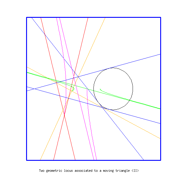
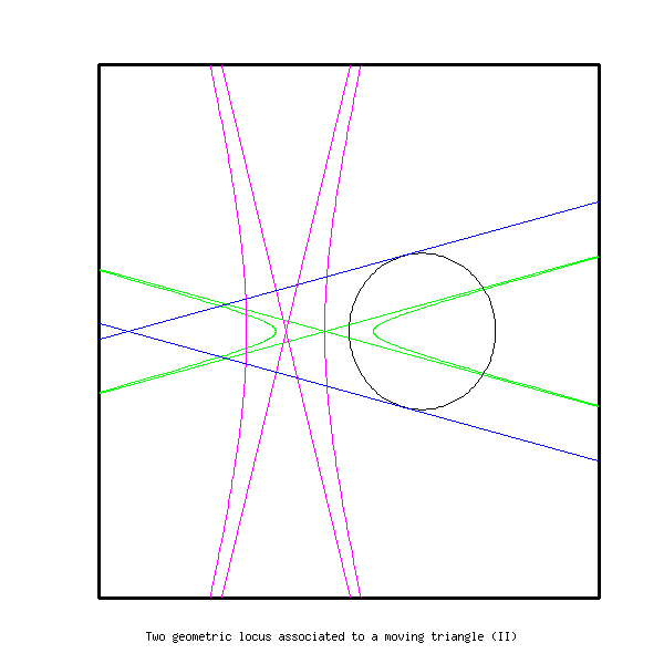
Program ex18, file geom.cmd
In this program we consider a circle with two fixed tangent lines ![]() ,
, ![]() .
a third tangent line
.
a third tangent line ![]() is moving on the circle and
the three lines define a
moving triangle whose sides are tangent to the circle. We
are interested by the locus of the intersection of the medians and the
locus
of the intersection of the mediatrices.
is moving on the circle and
the three lines define a
moving triangle whose sides are tangent to the circle. We
are interested by the locus of the intersection of the medians and the
locus
of the intersection of the mediatrices.
The program draws a sequence of triangles around the circle with their medians and mediatrices. The intersections points are put in two polygons. Each time a new triangle is drawn, a vertex of each polygon is added.
It seems from the result of this program that the two locus are hyperbolas. The reader can try to prove this.
To run the program, when geom.cmd is loaded, type the commands :
 - funct -> clear X
 - funct -> ex18
:ex18
1
0
-1
point A
point O
point O1
point O2
point A1
point A2
point P
point P1
point Q1
point Q
point M
vector U
line l
line lp
line lq
line ort
line ort2
line med1
line med2
polyg Pol 362
polyg Pol2 362
circle C
circle C2
coord O 0 0
coord C O 0.5
d=-3
coord A -2 0
dist A O
d2=sqrt(dist_p*dist_p-0.25)
coord C2 A d2
inters_cc C C2 P Q
span_l lp P A
span_l lq Q A
defframe f
frame f -2.2 1.2 -1.7 1.7 5 5
setframe X f noax
setcolor X black
title X f Two geometric locus associated to a moving triangle (II)
dt=pi/180
subex18
destroy f
destroy A
destroy A1
destroy A2
destroy O
destroy O1
destroy O2
destroy P
destroy P1
destroy Q
destroy Q1
destroy M
destroy U
destroy l
destroy lp
destroy lq
destroy ort
destroy ort2
destroy med1
destroy med2
destroy C
destroy C2
destroy Pol
destroy Pol2
;
;
;
;
:subex18
1
0
-1
j=-1
do i 0 361
j=j+1
a=i*dt
coord M 0.5*cos(a) 0.5*sin(a)
coord U -sin(a) cos(a)
coord l M U
inters l lp P
setcolor X blue
draw l X f
draw lp X f
draw lq X f
trace 1
b=retval-1
if= b XXX
inters l lp P1
inters l lq Q1
b=1-retval
if= b XXX
trace 0
XXX:
middle A P1 A1
middle A Q1 A2
ortholine lp A1 ort
ortholine lq A2 ort2
setcolor X red
draw ort X f
draw ort2 X f
span_l med1 Q1 A1
span_l med2 P1 A2
setcolor X orange
draw med1 X f
draw med2 X f
inters med1 med2 O1
inters ort ort2 O2
show O1
coord Pol j point_x point_y
show O2
coord Pol2 j point_x point_y
sleep 20
setcolor X white
draw l X f
draw ort X f
draw ort2 X f
draw med1 X f
draw med2 X f
setcolor X green
draw Pol X f 0 j
setcolor X violet
draw Pol2 X f 0 j
setcolor X black
draw C X f
setcolor X blue
draw lp X f
draw lq X f
setframe X f noax
enddo
The locus of the intersections of medians is the green curve. The
locus of the intersections of mediatrices is the violine one. The final
result is shown on figure 39. An intermediate result is represented on
figure 38.
Program trans3d, file geom.cmd
In this program we consider the following transform of the plane
The successive transforms are drawn successively on the same window. The analogous program trans3c will not erase the previous transform of the circle before drawing a new one.
The program needs 3 arguments : the constants ![]() ,
, ![]() , and the number
of transforms.
, and the number
of transforms.
To run the program, when geom.cmd is loaded, type the commands :
 - funct -> clear X
 - funct -> trans3d 17 40 40
:trans3d
4
0
-1
transform_gen T x+sin(#1*y)/#2 y+cos(#1*x)/#2
xrange xr 1 10001
fix_xrange xr 0 pi/5000
function X xr
function Y xr
fill_func X cos(x)
fill_func Y sin(x)
polyg P 10000
polyg_funct P X Y
defframe F
if> #1-4 XXX
frame F -4 4 -4 4 2 2
goto YYY
XXX:
frame F -2 2 -2 2 1 1
YYY:
setframe X F
title X F 100 successive transforms of a circle by a transformation
do i 1 #3
echoi i
setcolor X red
act T P P
draw P X F
sleep 10
setcolor X white
draw P X F
setcolor X black
setframe X F
enddo
echo \n
setcolor X red
draw P X F
destroy P
destroy F
destroy T
destroy xr
;
In the first figure below the result with ![]() ,
, ![]() is represented, for 40 transforms.
In the next figure we take
is represented, for 40 transforms.
In the next figure we take ![]() ,
, ![]() and 40
transforms.
and 40
transforms.
![]()